
Software power draw on ARCHER2 - the benefits of being an RSE
By Andy Turner (EPCC) on October 10, 2022
Tags:
One of the big benefits of being a research software engineer (RSE) providing general support for a compared to a researcher or being focussed on a specific project is the ability to take a step back from the specific aspects of particular software and look at the more global view of software.
I really enjoy that an RSE role gives me the ability to have a holistic view of software use patterns and how such data can be used to improve the service for researchers and - for the case I am going to discuss below - how we can use the data to try and make the service more efficient environmentally.
I think one of the key benefits that RSEs bring to the research community is this ability to have a wider view of the research and software landscape than is possible for researchers who are necessarily focussed on their particular research problem. They can bring lessons learned and ideas from other research areas to help the researchers they are currently working with. For me, this breadth of experience is also one of the best parts of being an RSE - the diversity of work and the feeling that you are creating links between different researchers are some of the things I find most satisfying about my RSE role.
One of the projects I have been working on over the past few months that has allowed me to take this high-level view of software on the ARCHER2 UK national supercomputing service is the HPC-JEEP project funded by the UKRI DRI Net Zero Scoping Project. The idea behind HPC-JEEP is to look at what energy usage data we can extract on a per job basis from HPC facilities and what types of analyses this energy data can currently support. This information can then be used to plan future activities about how you might optimise an HPC service in terms of minimising emissions per unit of research. The HPC-JEEP project includes two HPC services as testbeds for this analysis: ARCHER2 (supported by EPCC at the University of Edinburgh) and DiRAC COSMA (supported by the ICC at Durham University).
The initial report from HPC-JEEP on how we extract energy data and some initial exploratory analysis of energy use by different research areas and software on the HPC systems has recently been published on Zenodo along with the dataset that includes the raw and analysed per job data from ARCHER2 and DiRAC COSMA along with the analysis scripts used for the report. This plot from the report compares the percentage energy use and percentage node hour use broken down by research areas on ARCHER2. The labels above the bars show the percent difference between the energy use and node hour use columns.
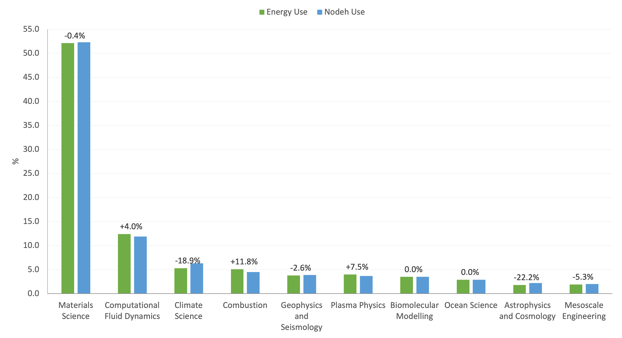
If all software on ARCHER2 consistently drew the same amount of compute node power we would expect to see no difference between the percentage energy use and the percentage node hour use. Where the differences are large, some behaviour of the users (e.g. not using all compute cores on a node) or some aspect of the application (e.g. it is IO-bound so is not using compute cores consistently) is leading to these discrepancies.
As part of HPC-JEEP we have recently been able to extract per-job mean node power draw statistics and then break these down by research area and software. The plot and table below show the distribution of node power draw on ARCHER2 weighted by the number of node hours used for each job and broken down by research area for July 2022. (We only list areas that have greater than 1% use in the period.)
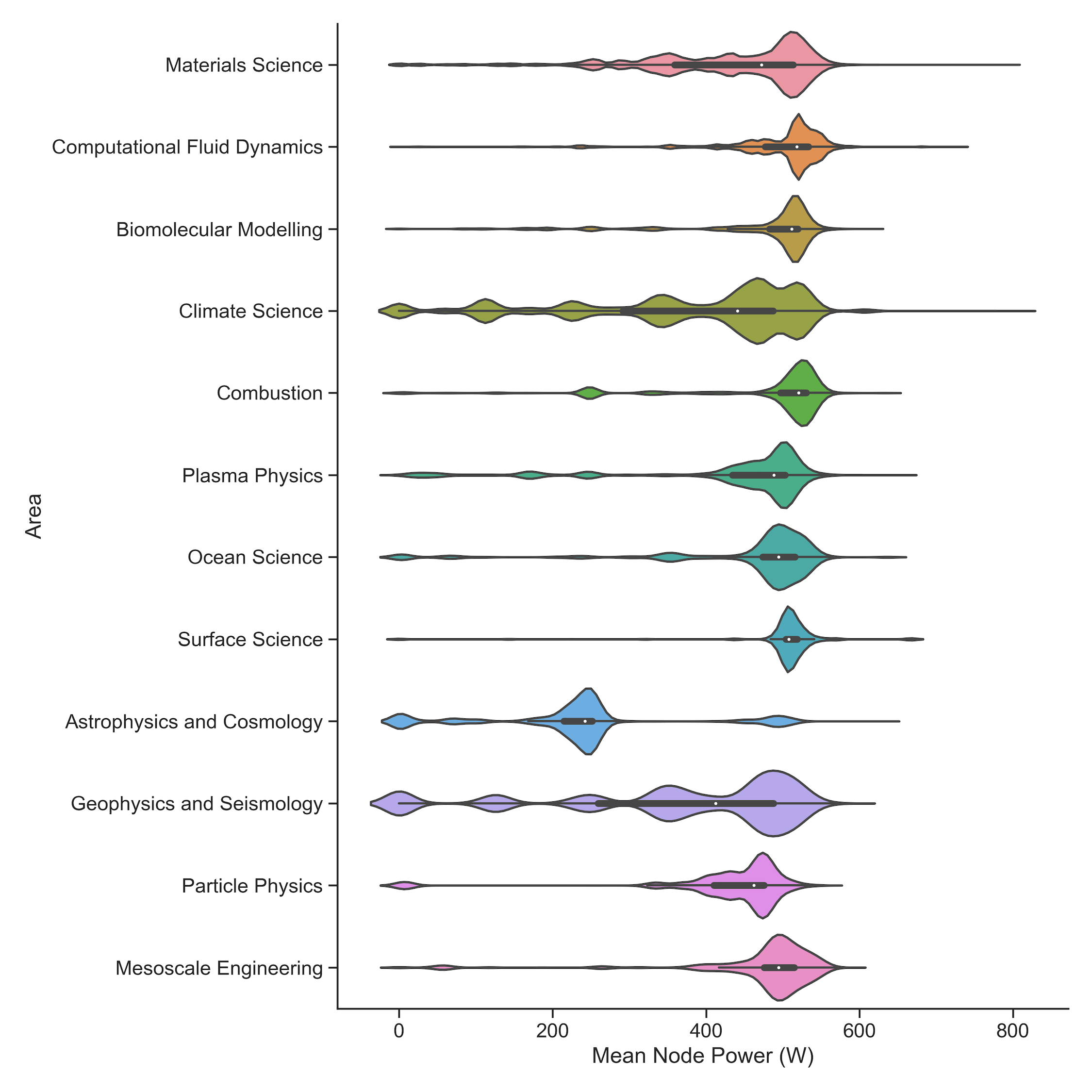
Distribution of node power draw (in W) weighted by usage and broken down by research area (July 2022, areas greater than 1% use):
| Area | Min | Q1 | Median | Q3 | Max | Jobs | Nodeh | PercentUse | Users | Projects |
|---|---|---|---|---|---|---|---|---|---|---|
| Overall | 0.0 | 366.4 | 489.9 | 518.8 | 802.9 | 324624 | 3383514.6 | 98.1 | 567 | 87 |
| Materials Science | 0.0 | 356.3 | 473.4 | 514.0 | 795.6 | 220307 | 1558728.8 | 45.2 | 217 | 16 |
| Computational Fluid Dynamics | 0.0 | 476.3 | 518.2 | 536.1 | 729.4 | 8786 | 565598.2 | 16.4 | 84 | 20 |
| Climate Science | 0.0 | 229.8 | 431.1 | 482.3 | 802.9 | 45959 | 257226.6 | 7.5 | 46 | 2 |
| Biomolecular Modelling | 0.0 | 482.9 | 511.5 | 520.1 | 763.0 | 7344 | 220833.3 | 6.4 | 29 | 2 |
| Combustion | 0.0 | 478.3 | 517.1 | 530.5 | 632.9 | 996 | 162618.5 | 4.7 | 21 | 3 |
| Plasma Physics | 0.0 | 406.0 | 492.7 | 503.7 | 649.6 | 2049 | 140584.1 | 4.1 | 20 | 5 |
| Astrophysics and Cosmology | 0.0 | 202.1 | 242.1 | 251.6 | 627.4 | 387 | 113067.1 | 3.3 | 6 | 1 |
| Ocean Science | 0.0 | 472.1 | 494.4 | 516.0 | 636.0 | 2493 | 104284.1 | 3.0 | 25 | 2 |
| Geophysics and Seismology | 0.0 | 256.3 | 412.7 | 491.5 | 583.0 | 25224 | 61505.2 | 1.8 | 16 | 2 |
| Surface Science | 0.0 | 502.4 | 507.5 | 518.9 | 666.8 | 145 | 55262.7 | 1.6 | 2 | 1 |
| Particle Physics | 0.0 | 410.2 | 464.5 | 475.5 | 552.5 | 155 | 41538.4 | 1.2 | 5 | 3 |
| Mesoscale Engineering | 0.0 | 472.1 | 494.0 | 514.6 | 583.9 | 1416 | 34961.9 | 1.0 | 14 | 1 |
The mean node power draw is computed by taking the total energy used by the job and dividing it by the runtime and the number of nodes used. You can see clear differences in terms of the node power draw that fit into three broad categories:
- High node power draw: Computational Fluid Dynamics, biomolecular modelling, combustion, surface science, mesoscale engineering
- Medium node power draw: materials science, plasma physics, ocean science, particle physics
- Low node power draw: climate science, astrophysics and cosmology, geophysics and seismology
There is also the outlier of the astrophysics and cosmology area which has extremely low power draw. Further investigation reveals that this is beacuse all the jobs in this category (which comes from a single project on ARCHER2) only use half of the compute cores on a compute node - presumably to make more memory capacity or bandwidth available per process/thread for the application.
We can gain a different perspective on node power draw by breaking down the distribution by the software used in the job rather than research area. The plot and table below show this breakdown. Again, the per job node power draw is weighted by node hour use to give proper weight to the applications and jobs according to their usage on ARCHER2. (We only list software that have greater than 1% use in the period.)
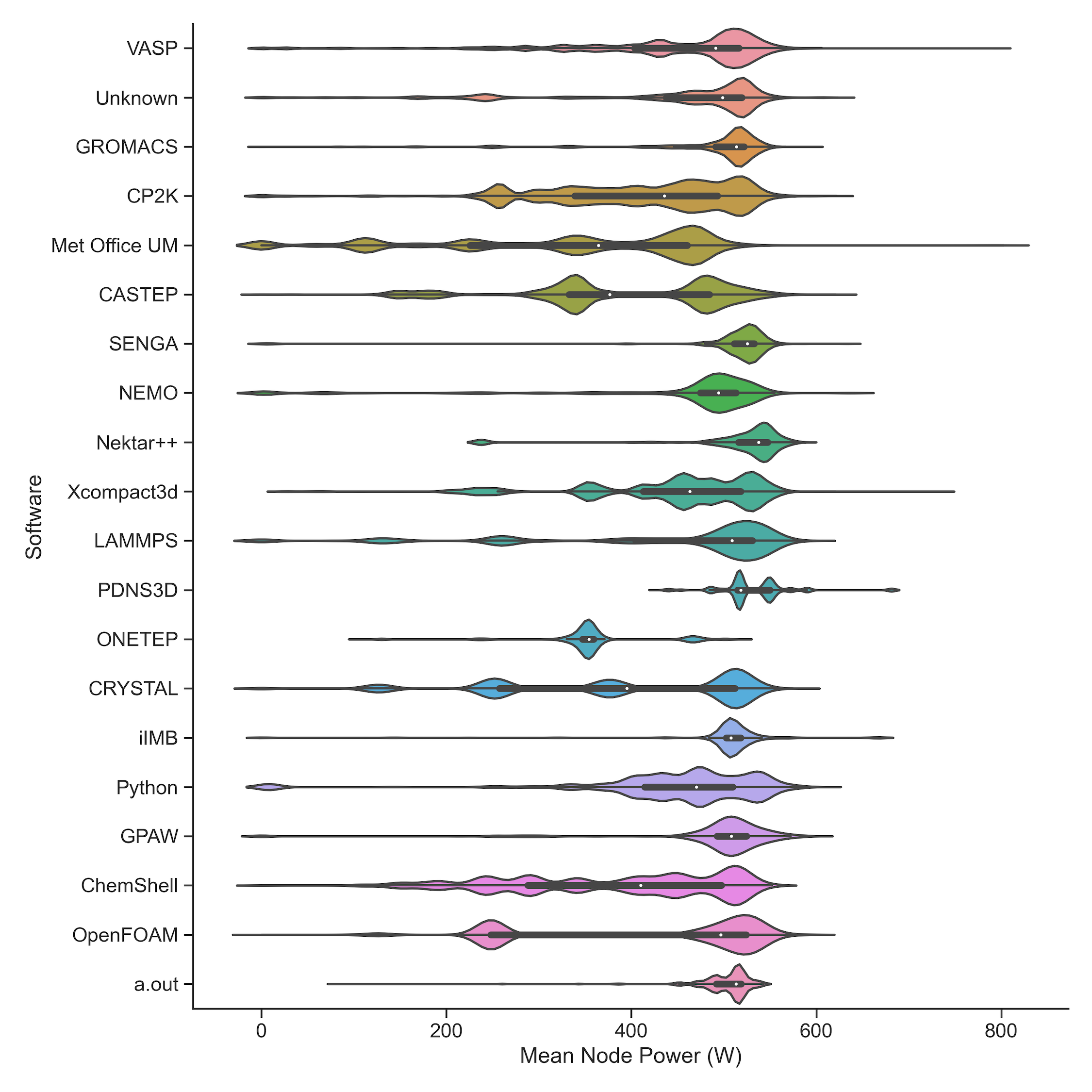
Distribution of node power draw (in W) weighted by usage and broken down by software (July 2022, software greater than 1% use):
| Software | Min | Q1 | Median | Q3 | Max | Jobs | Nodeh | PercentUse | Users | Projects |
|---|---|---|---|---|---|---|---|---|---|---|
| Overall | 0.0 | 353.7 | 472.3 | 508.0 | 802.9 | 324624 | 3383514.6 | 98.1 | 567 | 87 |
| VASP | 0.0 | 403.5 | 477.9 | 505.0 | 795.6 | 55325 | 881158.3 | 25.5 | 111 | 11 |
| Unidentified | 0.0 | 303.2 | 348.2 | 455.5 | 623.3 | 38104 | 500228.3 | 14.5 | 181 | 62 |
| GROMACS | 0.0 | 446.5 | 511.5 | 530.3 | 763.0 | 4648 | 235137.2 | 6.8 | 32 | 7 |
| CP2K | 0.0 | 393.7 | 489.2 | 516.1 | 621.6 | 4609 | 205745.1 | 6.0 | 40 | 8 |
| Met Office UM | 0.0 | 216.3 | 331.6 | 434.4 | 802.9 | 41216 | 199483.0 | 5.8 | 26 | 1 |
| CASTEP | 0.0 | 461.3 | 493.2 | 519.6 | 629.7 | 117059 | 127935.5 | 3.7 | 29 | 7 |
| SENGA | 0.0 | 501.7 | 512.3 | 530.5 | 632.9 | 105 | 110031.9 | 3.2 | 6 | 2 |
| Xcompact3d | 0.0 | 380.4 | 434.5 | 496.4 | 729.4 | 440 | 97612.1 | 2.8 | 10 | 4 |
| NEMO | 0.0 | 340.0 | 389.3 | 462.2 | 636.0 | 2319 | 93777.6 | 2.7 | 18 | 3 |
| Nektar++ | 0.0 | 427.1 | 481.6 | 511.5 | 585.5 | 1376 | 91555.0 | 2.7 | 9 | 4 |
| LAMMPS | 0.0 | 262.2 | 421.6 | 497.8 | 595.0 | 7141 | 85953.6 | 2.5 | 33 | 11 |
| CRYSTAL | 0.0 | 256.3 | 496.7 | 514.4 | 574.2 | 1285 | 80825.0 | 2.3 | 9 | 3 |
| ONETEP | 0.0 | 284.2 | 356.2 | 478.4 | 517.7 | 364 | 77866.0 | 2.3 | 4 | 1 |
| PDNS3D | 0.0 | 495.8 | 547.0 | 552.3 | 681.3 | 41 | 72562.7 | 2.1 | 1 | 1 |
| ChemShell | 0.0 | 392.8 | 450.5 | 504.2 | 551.6 | 1187 | 55332.9 | 1.6 | 13 | 3 |
| iIMB | 0.0 | 503.0 | 507.6 | 522.2 | 666.8 | 124 | 53534.2 | 1.6 | 2 | 1 |
| R-matrix | 1.8 | 201.5 | 220.2 | 228.1 | 300.1 | 23 | 50437.3 | 1.5 | 1 | 1 |
| Python | 0.0 | 379.7 | 445.1 | 484.3 | 602.6 | 714 | 50263.5 | 1.5 | 13 | 12 |
| GPAW | 0.0 | 471.7 | 494.7 | 510.1 | 596.4 | 23349 | 44793.0 | 1.3 | 3 | 1 |
| OpenFOAM | 0.0 | 424.5 | 500.3 | 524.0 | 588.5 | 869 | 42845.0 | 1.2 | 23 | 10 |
| a.out | 0.0 | 474.8 | 491.2 | 511.3 | 542.8 | 419 | 35326.8 | 1.0 | 6 | 6 |
The plot of the distributions shows some interesting features. In particular:
- A number of codes clearly show multiple distinct use types that fall into different node power use regimes. This is particularly distinct for the Met Office UM and CRYSTAL. Further investigation is needed to see if these different power use regimes correspond to different levels of population of nodes with process/threads (i.e. not using all cores on a node) or if it is due to something else.
- Some codes look like they are used with either all cores in a node populated with processes/threads or with half the cores populated. Clear examples of this are CASTEP and OpenFOAM.
- Many codes seem to populate all the cores with processes/threads but still have different levels of total power that they can draw. For example, compare Nektar++ with NEMO, both look like they are using all cores on a node consistently but the node power draw for NEMO is generally lower than that for Nektar++.
- Some codes have a very broad distribution of power draw - for example, CP2K and Xcompact3d. In these cases, breaking down particular code use by project or research area may be able to shed light on how different communities are employing these codes.
We are looking into understanding this data further and, in parallel, working to understand how the performance of application benchmarks vary with different power caps on the compute nodes. The combination of these different investigations will hopefully provide data that we can use to potentially optimise the energy efficiency of applications on ARCHER2 and DiRAC COSMA. The next steps for the HPC-JEEP project are to investigate HPC charging units that include a component of energy use (rather than just being based on residency, as most current HPC charges do) and propose ways of reporting energy use (and potentially associated emissions) back to users to allow them to undestand how much energy they are using in their use of HPC and give them a baseline from which they can measure any improvements in energy efficiency.
Being an RSE supporting the ARCHER2 service allows me to take this type of broad view of usage of the service that I would not have if I was focussed on one particular area of research.